Calc spreadsheet file used in video: Right-click to download file
To apply a custom format, first select the cell or range of cells then right-click and choose Format cells.
Choose the category that fits the format you want to create.
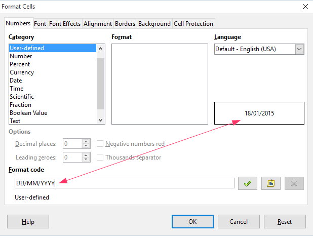
For example a date format. choose Date for the category then in the Format code text box type the format using date codes for the month, day and year.
DD/MM/YYYY will format the cell so that a date will display 01/01/2015 with 2 digits for day and month and 4 for the year, and forward slashes separating them.
The codes you use for dates depends on the locale setting of your computer. For example if the computer is set to German locale the format for day/month/year would be TT/MM/JJJJ.
The codes which can be used for dates and locales can be found on the reference page here
A preview of the custom date format is displayed on the middle right column of the Format cells dialog:
You can add a comment to the new format by clicking the Edit comment button:

When the format is selected in the Format window the comment will appear below the format code text box.
Click the check button to add the format. Then click ok.

When a date is entered into the cell it will take on the custom format.
When you create a custom date format you can use any character for a separator between the month, day and year. If the separator is the same as a date code like a Y, you would have to type one more than the maximum number used in the code.
The dates with times can be formatted in a variety of ways. to display the days/months/years then hours minutes seconds with fractions of a second the format dd/mm/yyyy hh:mm:ss.00 would be used. To show AM or PM at the end of a time use AM/PM at the end of the format hh:mm:ss AM/PM.
Number formats use placeholders such as the number sign # for significant digits and zero 0 for insignificant digits. a zero displays zeros if there are fewer numbers than the number format.
The question mark ? is used to represent the number of digits to include in a fraction.
If the number contains more digits to the right of the decimal then there are place holders it will be rounded. If there are more numbers to the left of the decimal than the format indicates, all the numbers will be displayed.
A comma, period (Full Stop), or a blank space can be used as a thousand separator. The separator can also be used to show numbers truncated by 1000s. For example the number 25,000 with the format #,
would display as 25.
To display Text mixed with numbers place a double quote before and after the text. A backslash \ can be used for a single character. for example #, "Thousand" would display 25 Thousand in a cell which contained the number 25,000. #.#\m would display 8.9 m in a cell which contained 8.9.
Eight different colors can be applied to the numbers in cells by using the color name in square brackets before the format.
[BLUE] ##.0#
The currency format for the speadsheet is determined by the regional setting of the operating system. You can apply a custom currency by typing the currency symbol with the format for example: £ #,###.00
Or you can use the locale code for the country in square brackets. [$£-809] #,###.00. The locale code for any country can be found by choosing currency in the category window then in the format dropdown choose a currency. The format will appear in the format code, the locale code for the country will appear in square brackets. Copy the code to use it in a custom format.
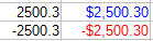
Conditional operators can be used to determine the color of a number by putting the operators in square brackets:
[RED][<0]-[$$-409]#,###.00;[BLUE][$$-409]#,###.00
Results: