
Calc spreadsheet file used in video: Right-click to download file
The Gantt Chart being created here is a simple type where the projects are independent of one another.
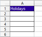
In column A set up a holiday table for Holidays in the month. The following example has a table for up to 4 holidays in the month in cells:
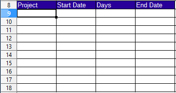
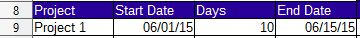
Next create a table for projects with columns for the Project Name, Start Date, Days to complete, and End Date. In the example below the table was created starting in cell A8:
In the next cell to the right of the End date field header, type the first date for the month. select the date then drag the fill handle to the right to fill in the days of the month:

To place the days of the week on top of the dates, in the cell directly above the first date:
Type = (equals)
click the date cell Below.

Press Enter
Right-click on the cell and choose Format Cells
In the dialog type into the Format code input box ddd to get the day of the week abbreviation:
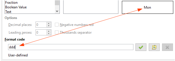
Click OK.
Click the cell to select it then drag it to the right to fill the month.
Format the date cells with border and background colors if desired
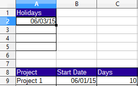
type the dates for any holidays for the month in the Holidays table. Fill at least 1 project, Start Date, and number of days for the project.
For the End date cell the WORKDAY.INTL function is used.
This function will return the date before or after a specified number of workdays. There are parameters for Weekend days (specified with a code), and holidays (specified with an array of dates).
In the End date cell add the code:

In the first parameter has the Start Date in B9, Second parameter is the number of days in B10. The third parameter is the weekend, 1 is the code for Saturday and Sunday. The final parameter is an array containing 2 holiday dates from the Holiday table, for these the rows must be locked in order to copy the formula down the column. The date returned is the date after the number of workdays so 1 is subtracted from the date to get the actual last day of the project.
In order to be able to have empty cells to fill in more projects the WORKDAY.INTL function should be placed in an IF function with the ISNUMBER function testing the Days cell. If no number was entered into the Days cell yet a blank cell is returned for the End Date:

The Result:
Now the formula can be copied down column D with the fill handle to Accommodate more projects.
The formula for creating the chart bars (cell E9 in the example) is inside an IF statement which first tests whether the date in the cell is within the project dates in B9 and D9, an And statement is used for the test. The And statement also test if there is a date in D9. If theres no date in D9 or the date is not within the project start and end dates an empty string is returned.
If the date is within the project date then another IF statement will test if the cell date is a workday or non-workday(holiday or weekend).
The NETWORKDAYS.INTL function is used to test whether the date in the cell is a holiday or weekend. The function returns the number of workdays between 2 dates, in this instance the 2 dates are the same, the date of the cell. So if the date is a holiday it returns a 0 if it's a workday it will return 1. The other 2 parameter are the weekend code and the holiday array.
The second IF statement will return a W if it's a workday and an H if it's a non-workday.

Click in the cell with the formula and Drag the fill handle to the end of the dates. Then drag the fill handle down the rows to however many rows you desire for more projects.
Select the area which contains the formula then press the Conditional Formatting Button.
In the dialog Condition 1 should be Cell value is equal to. In the text box type "W".

A style will be created with the text color the same as the background color, so that the text will be invisible. the Workdays will have a green background and the weekends will have a blue background, so they can be distinguished easily.
in the Apply Style dropdown choose New Style...
Name the style (for the example the name is Green)
Under the font effects tab change the font color to light green.
Under the Borders tab/line arrangement choose all four borders.
Under the Background tab choose light green as the background color.
Press OK
Click Add to add another condition. in the cell value is equal to text box type "H".

in the Apply Style dropdown choose New Style...
Name the style (for the example the name is Blue)
Under the font effects tab change the font color to light blue.
Under the Borders tab/line arrangement choose all four borders.
Under the background tab choose light blue as the background color.
Press OK
Press OK on the conditional formatting dialog.
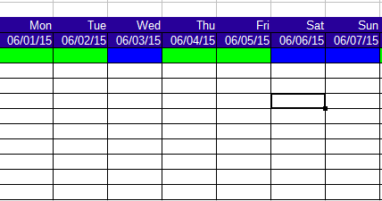
Result:
Weekend Codes for the WORKDAY.INTL and NETWORKDAYS.INTL function