Calc spreadsheet file used in video: Right-click to download file
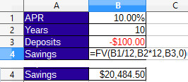
The Fv function provides a way to calculate how much a savings account with a fixed interest rate will yield after a given amount of time. The function has 4 parameters.
For example, a savings account is opened which has an APR of 10%, a deposit of $100 is made into the bank for 10 years:
The PMT function can be used to determine the amount of payments to reach a certain goal. for example a goal of 50,000 is desired for a savings account with a 10% fixed interest rate for 10 years. To find how much the monthly deposits would be to achieve this you can use the PMT function:
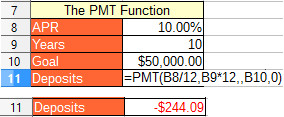
The first parameter, Rate is divided by 12 to get the periodic rate.
The next parameter, NPER, the number of years is multiplied by 12 to get the number of monthly deposits.
Third parameter is PV, present value, if there was already a balance in the bank it would be put here, but in this example it's presumed that the savings account has no money in it, so the parameter is left blank.
The fourth parameter is FV, the future value, This is the goal amount that is sought.
The final parameter is Type, This is 0, the payments are at the end of each period.
With this formula you can change the Goal amount find a suitable deposit amount for your budget.
Some more complicated calculations are better done with Calc's Goal Seek feature, for example a car loan, the bank offers 5 year loan at 3.9% and you want to calculate the price of a car that would fit your budget. First create a table with the APR, The years to pay and a guess for the loan amount in the example, $25,000. The payment function is entered as a negative in order to calculate a positive result for use with Goal Seek: =-PMT(B3/12,B4*12,B2)
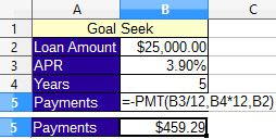
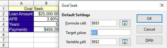
Suppose you couldn't afford more than a payment of $400 a month. To calculate the price of the car you can buy for that payment:
Click the cell with the payment formula.
Either go to the Tools menu and choose Goal Seek
Or use the menu shortcut hold down Alt and press T G
In the dialog make sure the formula cell is the cell with the payment formula.
In the Target Value type the amount of payments you want to pay.
Click the textbox next to Variable cell then click the Loan Amount cell on the spreadsheet.
Click OK
Goal Seek will calculate how much the loan would be for $400 a month payment. Another pop up will appear with the result and ask if the result should be inserted into the cells.
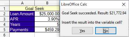
You can try out different payment amounts by bringing up the Goal Seek dialog again.
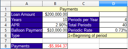
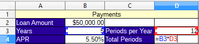
The best way to use the payment function is with a table that contains the full details of the interest rate and the number of periods per year. Some loans are quarterly rather than monthly, so for full versatility a table something like the following example should be used:
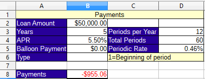
By arranging a table in such a way, any value for the parameters can be changed without changing the formula. In D5 the periodic rate is calculated by dividing the APR in B4 by the periods per year in D3:
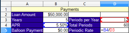
In D4 the total periods is calculated by multiplying the Periods per Year in D3 by the Years for the loan in B3:
This makes the PMT function simpler as there's no need to divide the APR or multiply the Years parameters:
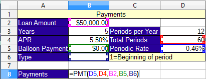
By arranging the table this way you can change the Years, Periods per Year, APR, Balloon Payment, and Type to adapt to any loan.
For example a $200,000 loan for 10 years with a 2.9% APR to be paid quarterly, with a balloon payment at the end of $10000 can be easily entered into the cells with changing the formula at all: