IFNA

Calc spreadsheet file used in video: Right-click to download file

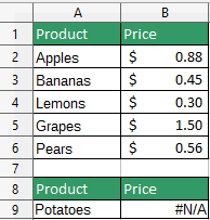
the IFNA function can be used to return a value if an #N/A (not available) error occurs from a function. for example in the following table a product is typed into cell A9 and by use of a VLOOKUP function the price is returned in B9, but if the product is not in the table an #N/A error occurs:

by using the IFNA function a useful message can be returned to the user when the error occurs. the IFNA function takes 2 parameters:

• Value: this is formula that is checked for an #N/A error, if there is no error the value from the formula is returned.
• Alternate_value: this is a value or formula that is returned when an #N/A error is detected.

In the above example to have the cell display a message when the #N/A error occurs, you would put the vlookup function into the first parameter of the IFNA function, then in the second parameter a message:

Another way to use IFNA is to put another function in the second parameter, for example if you wanted to search 2 different tables with VLOOKUP:

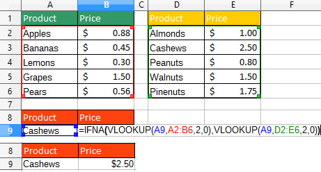
The first parameter of the IFNA functions contains the VLOOKUP function which searches through the first table for the item in A8, if it doesn't find the item, the VLOOKUP function in the second parameter executes and searches through the second table for the item then returns the price:

If there were more than 2 tables another IFNA function can be added to the second parameter of the first IFNA function:

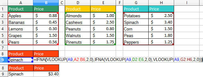
=IFNA(VLOOKUP(A8,A2:B6,2,0),IFNA(VLOOKUP(A8,D2:E6,2,0),VLOOKUP(A8,G2:H6,2,0)))
For long formulas like this use the define names feature to make them smaller and more readable.
For example if the function VLOOKUP(A8,A2:B6,2,0) is defined as findfruit, (VLOOKUP(A8,D2:E6,2,0) is defined as findnuts and VLOOKUP(A8,G2:H6,2,0) is defined as findveg the formula could be rendered as:
=IFNA(findfruit,IFNA(findnuts,findveg))