
Calc spreadsheet file used in video: Right-click to download file
Conditional formatting will allow you to define formatting styles to cells according to certain conditions.
To apply cell formatting click a cell or highlight a range of cells then press the Conditional Formatting button on the toolbar:

Or use the shortcut: hold down Alt and press O O C
The conditional formatting dialog appears.
To apply formatting based on a cell value:
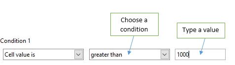
Under where it says "Condition 1": Choose "Cell Value is" in the drop-down
In the next drop-down choose a condition then in the text box next to it type in a value.
In the drop-down next to where it says apply style choose a style or click New Style... to create a new style:
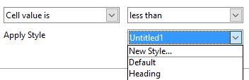
If New Style is chosen a Cell Style dialog appears and you can create a new cell style for the cell or cells that match the condition.
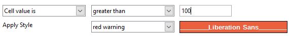
When a style is created or chosen a preview appears in the box on the right:
Click the Add button to add more conditions to the cell or cell range, or the Delete button to delete conditions.
Under where it says "Cell Range" a different cell range can be chosen by clicking in the text box then click a cell or drag and highlight a range of cells.
Click OK when finished.
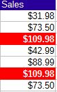
Cells formatted with the condition more than $100:
Color scale formatting applies a 2 or 3 color gradient to a range of values based on the values of each cell. Drag and highlight a range of cells then press the Conditional Formatting:Color Scale button:

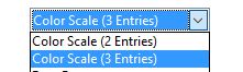
In the dialog that appears choose 2 or 3 entries in the drop-down at the top. 3 entries is the default:
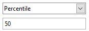
If 3 Entries are chosen, type in the percentage where the center color should be located in the gradient scale. the default is 50%:
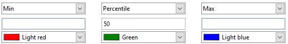
Then choose the colors for the min, max and (if 3 entries are chosen) the center values.
Click OK
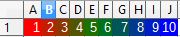
An example of a color scale applied to a range of cells with the values 1 to 10 and the center point at 50%:
Data bar formatting applies horizontal bars to the background of the cells indicating the percentage of the value in the cell compared to the largest value in the range selected. If there are negative amounts the bars will be colored red going in the opposite direction:
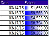
To apply data bars to cells, drag and highlight a range of cells then press the Conditional Formatting:Data Bar button:

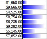
A dialog will appear, The default bars will be Blue for positive values and red for negative, to change the colors and for other options press More Options. In the More Options dialog you can choose to have only the bars display, this is useful if you have a copy of the values in a column next to the values:
When your finished with the More Options dialog click OK
Click OK in the data bar dialog
Icon set will place an icon next to the values in the cells in a range depending on their relative value.
To apply an Icon set to a range of cells, drag and highlight a cell range then press the Conditional Formatting:Icon set button:

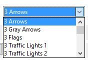
In the dialog that appears choose the type of icon you want displayed in the drop-down on the right, the default is 3 arrows:
Choose the point at which the icons should change in the text boxes to the right of the more than or equals signs:
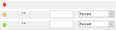
You can choose whether the conditions to display the icons are relative to a percentage, value or formula in the drop-downs at the right. Percentage is the default.
Click OK.
An example of an Icon set applied to values 0 to 10 the icons were set to change at 25% and 75%:
Conditional formatting on a page can be Added, Edited and Removed by using the Manage Conditional Formatting dialog.
go to the Format Menu, choose Conditional Formatting then choose Manage.
OR use the shortcut:
hold down Alt and press O O M