
Calc spreadsheet file used in video: Right-click to download file
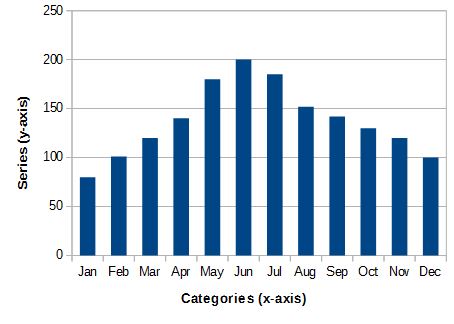
You will usually want to summarize data before making a chart. In chart lingo, series are the range of values, categories are the labels for the series. The x-axis is the horizontal axis, and the y-axis is the vertical. In this column chart the series data is aligned along the y-axis and the categories are aligned along the x-axis:
To create a chart select the range of cells to be represented in the chart.
Click the Chart button on the toolbar
Or in the Insert menu choose chart
Or shortcut: hold down Alt and press I A
A preview of the chart will appear along with the Chart Wizard which will take you step by step through the process of completing the chart.
You do not have to go through all the steps, click on the steps where you need to make modifications, if you are happy with the preview of the chart at any point press Finish. You can always edit it later if you change your mind.
These are the steps in the wizard:
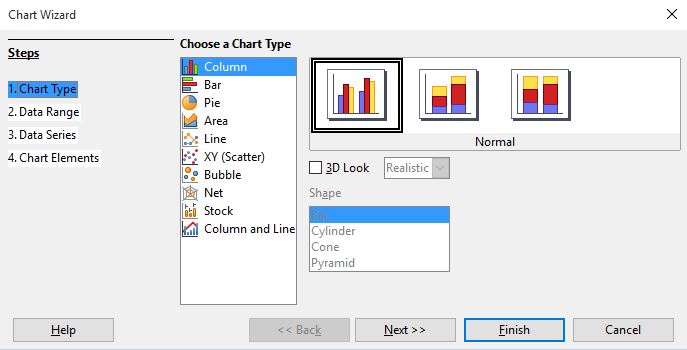
Step 1 - Chart Type:
There are a wide variety of charts available, select one that's appropriate for the data. The most common charts are:
Column and Bar charts have rectangular bars with lengths proportional to the values they represent.
Pie charts display percentage values as pie slices. They're used when you want to view items as a percentage of a whole.
Line Charts show values as points on the y axis (horizontal). They are best used to represent numbers which change over time.
There are several variants for each chart type represented in the window to the right.
Some charts types can be generated in 3D. Check 3D Look for a 3 dimensional chart. With 3D charts you can choose between a Realistic or Simple look and choose from different shapes.
Click Next.
Step 2 - Data Range:
Data range is the selected area of the table used in the chart. If you want to select a different area of the table then click the button to the right of the Data Range text box:

Then drag and highlight the area you want to include in the chart.
choose if you want the data series to be in columns or rows. by default First row as label and first column as label are checked. This means it will take the field names from the first row and the first column of rows as the labels used in the chart.
Click Next.
Step 3 - Data Series:
In this step you can add or remove a data series in your chart. By clicking on an item in the data window you can choose a range for the Border color, Fill color, Name and Y values. For example if your using a bar or column chart, click Fill color then click the button to the right of the input box under where it says Range for Fill color. Drag an highlight the row of amounts used for the series data, and you will get different colors on each bar.
Click Next.
Step 4 - Chart Elements:
Here is where you add a Title and Subtitle to the chart, you can also add text to the X and Y axis of the chart. The Z axis is only available if you have are creating a 3D chart.
Under where is says Display Grids, choose if you want grid lines displaying on the chart.
On the Right you can choose whether to display a ledgend and where it should be placed.
Clicked finished.
Calc is still in Chart Edit mode, in the toolbar area there are now buttons for editing the chart.
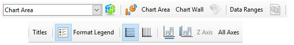
Click one of the buttons in the toolbar to modify different areas of the chart.
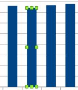
To format an item in the chart, click on it, if the item is a group, each item in the group will have a small square in at the center to indicate it's selected. Below is a column chart with all the bars selected:
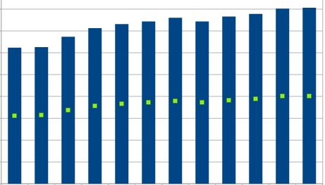
To selct an individual item in a group, like a single bar, after selecting the group, click on the individual item. Below is the same chart with one bar selected:
With the item or group selected, click the format button:

A dialog will appear where you can format the selection.
If have an individual item from a group selected and you want the complete group selected again, click in a blank area on the chart then click an item in the group.
To show data labels on the items in a chart (like the bars in a bar chart or the slices in a pie chart), right-click on the group and choose Insert Data Label.
the labels can be formatted by right-clicking on a label and choosing Format Data Label.
Other options like trend lines and x and y error bars are also available by right-clicking on a bar.
To go out of chart edit mode, click somewhere on the sheet outside of the chart.
You can move the chart by clicking on it and dragging it to a new location.
You can go back to edit mode at any time by double-clicking on the chart.