
Calc spreadsheet file used in video: Right-click to download file
Tables are made up of related rows and columns, they should be isolated from one another by empty cells.
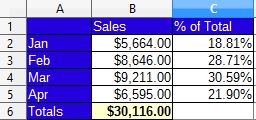
Tables should contain row and/or column headers to indicate what the values in the cells represent, in the following example the table contains Sales and % of Totals as column headers.
the months Jan - Apr and the Total are row headers:
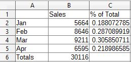
This table would look a lot clearer with formatting.
First, to format the headers so they stand out drag the mouse over A1 to C1, then press
Ctrl and drag down from A2 to A6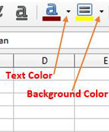
In the formatting toolbar click the arrow next to the background color button and choose a color, in this example I'm choosing a blue color. The text color should change to white, if not, or if you want a different text color press the arrow next to the text color button and choose a color.
The totals cell should have a different background color to distinguish it from the other values, so select the Totals cell, B6 then press the arrow next to the background color button again and choose a light yellow color.

Change the font in the total cell to bold by clicking the Bold Button in the toolbar.
Now to put a border around all the cells in the table to distinguish them from the other cells on the spreadsheet. First Drag from A1 to B6 then hold down Ctrl and drag from C1 down to C5.
Press the arrow next to the borders button:

Select All borders:
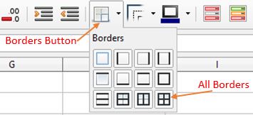
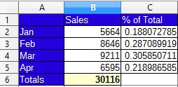
You can change the style of the borders by clicking the borders style button and choosing a style. The table should now look like this:
When you type a number in a cell on a new spreadsheet it takes on the default format and displays exactly as it is typed. You can format the number more specifically by using the number format buttons on the toolbar:
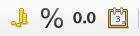
There are buttons for Currency, Percentage, Numbers, and Dates
Format the numbers in the "Sales" column by dragging from B2 to B6, then press the currency button:

Highlight the numbers in the "% of Total" column by dragging from C2 down to C5. Then press the percentage button.

Your table should now look like this:
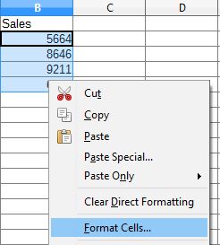
Another way to format cells and numbers which gives you more options is to highlight the cell or cells you want to format then right-click and choose "format cells". This brings up a format dialog. click the appropriate tab at the top to format Numbers, Fonts, Font Effects, Alignment, Borders and Background.
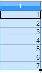
When you type a number, date or text which ends with a number into a cell you can easily fill adjacent cells with increments of the number or date. For example, type 1 into cell D1
press Enter
click D1 again to select it, in the lower right corner of the selection rectangle there's a small black square, this is known as the fill handle.
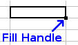
when you move the cursor over the black square it changes to a cross. when the cross appears, drag the handle down the column. The number will increment each row by 1.
You can also fill the months of the year. Type Jan into cell A8 and press Enter. Drag the fill handle across the sheet to D8.
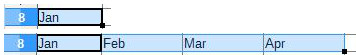
The days of the week also can be filled in this way.
One final tip for fomatting cells, if you have a cell formatted the way you want and you want to apply the format to other cells on the sheet, the clone formatting tool can be used.
Click a cell that has the formatting you want to copy, click the clone formatting button on the toolbar.

Then click the cell you want to apply the formatting to.
If you want to apply the format to several cells then click the cell with the format you want to copy and double-click the clone formatting button then click the cells where you want to apply the format, when your through, press Esc